Hochster’s Formula: How Topological Holes Become Betti Numbers
Published:
In my recently published article, the crucial bridge for converting a problem in algebra into a problem in topology is Hochster’s formula. In the paper, we discuss the formula briefly and we do provide an example of a simplicial complex so that the readers can get a sense of how the formula works, but regardless, it is an academic paper, so the formula isn’t really discussed in depth. I wanted to write an expository note on Hochster’s formula so that a mathematically mature reader with some undergraduate algebra and topology can hopefully understand the mechanism behind the formula better.
Introduction
A monomial ideal is an algebraic object and a simplicial complex is a combinatorial and topological object. At first, if you look at these two objects then you won’t really see any obvious reason to connect these two. However, there indeed is an elegant formula that connects the holes in a simplicial complex with a free resolution of a polynomial ring quotient. Hochster’s formula is the bridge, for squarefree monomial ideals.
More precisely, it turns certain Betti numbers, which are numbers that record the structure of a minimal free resolution, into dimensions of homology groups of simplicial complexes. This gives a remarkable connection from algebraic syzygies to topological holes and vice versa.
The goal of this post is to explain what this statement means through a small example, with as little machinery as possible. Naturally, I will not discuss the proof of the formula here.
Some necessary background
There’s some necessary vocabulary that we should build before attempting to explain Hochster’s formula. I will assume some basic understanding of undergraduate level group and ring theory and topology, however.
Let $S=k[x_1,\dots,x_n]$ be a polynomial ring over a field $k$. If we have $S=k[x_1,x_2,x_3,x_4]$, then elements of $S$ are polynomials such as $x_1x_3+x_2^2-x_4.$
A module over $S$, or an $S$-module, is similar to a vector space, except that the scalars in vector space are replaced by polynomials in $S$ rather than just numbers in the field $k$. So, for instance, if we can multiply a vector by a scalar such as 3 in a vector space, then in an $S$-module, we can multiply an element by a polynomial such as $x_1x_2+x_3$.
The polynomial ring $S$ itself is actually an $S$-module as well, since we simply multiply polynomials by other polynomials. A free $S$-module is an $S$-module that has a basis, much like a vector space has a basis. The basic examples are $S,S^2,S^3,\dots$. A free resolution is built out of these free modules.
Consider $I = (x_1x_3,x_2x_4) \subseteq k[x_1,x_2,x_3,x_4].$ The ideal has two generators, but those generators themselves satisfy a relation, namely $x_2x_4(x_1x_3)-x_1x_3(x_2x_4)=0.$
A relation like this among generators is called a syzygy.
A free resolution records this information by recording generators, relations among those generators, relations among those relations, and so on. For our example, a free resolution of $S/I$ has the form
\[0 \longrightarrow S(-4) \longrightarrow S(-2)^2 \longrightarrow S \longrightarrow S/I \longrightarrow 0.\]A module can have many free resolutions because we can simply always introduce more generators and relations, even if they are redundant. A minimal free resolution is one with these redundancies removed. Over a polynomial ring with its usual grading, the minimal graded free resolution is unique up to graded isomorphism, so the numbers appearing in it become invariants of $S/I$.
The notation $S(-d)$ is a standard way of recording a grading shift. It does not mean that the generator has degree $-d$. Rather, the basic generator of $S(-d)$ is placed in degree $d$. Therefore, $S(-2)^2$ records two free generators of degree 2, namely $x_1x_3$ and $x_2x_4$, while $S(-4)$ records one free generator in degree 4.
Equivalently, we could avoid the shift notation entirely and simply say our minimal free resolution has two generators in homological degree 1 and polynomial degree 2, and one generator in homological degree 2 and polynomial degree 4. This is the notation that I use in my recent paper, and also we will mostly use this latter viewpoint below as well.
The numbers of free generators in a minimal free resolution are called Betti numbers. The homological degree simply tells us the position in the resolution: in our example, $S$ is in homological degree 0, $S(-2)^2$ is in homological degree 1, and $S(-4)$ is in homological degree 2.
The total Betti number $\beta_i$ records only how many generators occur in homological degree $i$. A graded Betti number $\beta_{i,j}$ also remembers the ordinary polynomial degree $j$. For our example, $\beta_{1,2}=2$ means that there are two free generators in homological degree 1 and polynomial degree 2, corresponding to $x_1x_3$ and $x_2x_4$. Likewise, $\beta_{2,4}=1$ means that there is one free generator in homological degree 2 and polynomial degree 4, corresponding to the relation between those two generators.
We can keep even more information by remembering which exact variables occur rather than only their total degree. For a squarefree monomial, a subset $W=\lbrace i_1,\dots,i_r\rbrace$ corresponds to the multidegree of $x_{i_1}\cdots x_{i_r}$. The multigraded Betti number $\beta_{i,W}$ records a minimal free generator in homological degree $i$ with that particular multidegree. For our example again, $\beta_{1,\lbrace 1,3\rbrace}=1$ and $\beta_{1,\lbrace 2,4\rbrace}=1$.
If we forget which variables occur and remember only how many occur, then we recover the graded Betti numbers:
\[\beta_{i,j} = \sum_{\substack{W\subseteq[n]\\ \lvert W\rvert=j}} \beta_{i,W}.\]Hochster’s formula deals with these multigraded Betti numbers.
From a squarefree monomial ideal to a simplicial complex
A monomial is squarefree if no variable occurs with exponent greater than 1. For example, $x_1x_3x_5$ is squarefree, while $x_1^2x_3$ is not. A simplicial complex $\Delta$ on vertices ${1,\dots,n}$ is a collection of subsets of those vertices that is closed under taking subsets. Its elements are called faces.
There is a special kind of ideal associated to $\Delta$, which is called a Stanley–Reisner Ideal $I_\Delta$. A squarefree monomial $x_{i_1}\cdots x_{i_r}$ belongs to $I_\Delta$ when ${i_1,\dots,i_r}$ is not a face of $\Delta$. A nonface is a subset of vertices that is not a face, and a minimal nonface is a nonface whose proper subsets are all faces. The minimal nonfaces give the minimal monomial generators.
Consider the following simplicial complex, where the interior of the square is not filled in:
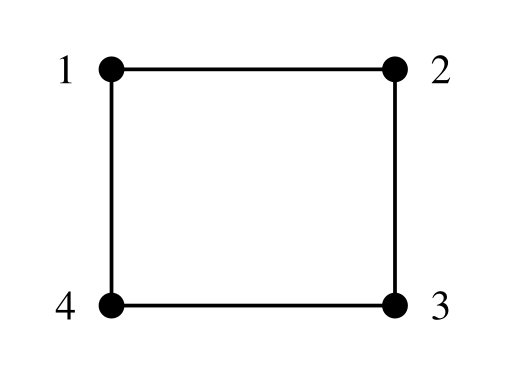
It consists of four vertices and the four boundary edges. The pairs ${1,3}$ and ${2,4}$ are the two minimal missing edges. Therefore $I_\Delta = (x_1x_3, x_2x_4).$
So the algebraic object from the previous section has a simple combinatorial picture: it is encoded by the boundary of a square!
Induced Subcomplexes
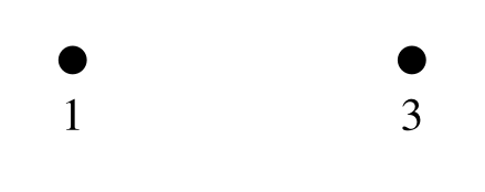
Hochster’s formula does not take $\Delta$ itself though; it takes the simplicial complexes obtained by restricting $\Delta$ to subsets of its vertices. Given $W \subseteq {1,\dots,n},$ the induced subcomplex $\Delta_W$ consists of all faces of $\Delta$ whose vertices lie entirely inside $W$. For instance, for our square, take $W = {1,3}.$ Since 1 and 3 are opposite vertices, there is no edge between them, so $\Delta_W$ consists of two disconnected points:
On the other hand, if $W={1,2,3,4}$, then $\Delta_W = \Delta$, which is the entire four-cycle. These two induced subcomplexes already contain all the topology we need to recover the nontrivial parts of the minimal resolution above.
Some homology that we need
Very roughly, homology provides a way to detect holes of different dimensions:
- $\widetilde H_0$ detects disconnectedness,
- $\widetilde H_1$ detects loops, and
- $\widetilde H_2$ detects two-dimensional holes.
The tilde notation denotes reduced homology. For our purposes, we just need to know that the main difference is in the dimension 0: if a space has $c$ connected components, then $\dim_k\widetilde H_0 = c-1$. Therefore, two isolated points have $\dim_k\widetilde H_0=1.$ A connected space has reduced $H_0$ equal to zero.
If we look at our unfilled square, then we can intuitively see that there is only one independent loop, so $\dim_k\widetilde H_1(\Delta;k) = 1.$ That is all the topology we will need for the example to follow.
Hochster’s formula
For a simplicial complex $\Delta$, let $k[\Delta] = S/I_\Delta$ be its Stanley–Reisner ring. For a subset of vertices $W$, Hochster’s formula says
\[\boxed{ \beta_{i,W}(k[\Delta]) = \dim_k \widetilde H_{|W|-i-1} (\Delta_W;k). }\]There’s a lot of notation here. Let’s unpack the formula.
To find a multigraded Betti number:
- Choose some vertices $W$.
- Look at the induced subcomplex on those vertices.
- Determine whether that complex has holes.
- Use the dimensions of those holes to determine where they appear in the resolution.
Example 1: the generators
Let’s return to the aforementioned ideal $I_\Delta=(x_1x_3,x_2x_4).$ Take $W=\lbrace1,3\rbrace$. Then the induced subcomplex consists of two isolated points:
It therefore has two connected components, so $\dim_k\widetilde H_0(\Delta_W;k)=1.$ Hochster’s formula gives
\[\beta_{i,\{1,3\}}(k[\Delta]) = \dim_k \widetilde H_{2-i-1} (\Delta_{\{1,3\}};k).\]The nonzero homology occurs in dimension 0, so we solve $2-i-1=0$, which gives us $i=1$. Therefore,
\[\beta_{1,\{1,3\}} = 1.\]The multidegree $\lbrace1,3\rbrace$ corresponds to the monomial $x_1x_3$, so topology has detected one of the minimal generators. The same thing happens for $W=\lbrace2,4\rbrace$, and it gives
\[\beta_{1,\{2,4\}} = 1.\]These correspond precisely to the two copies of $S(-2)$ in
\[0 \longrightarrow S(-4) \longrightarrow S(-2)^2 \longrightarrow S \longrightarrow S/I_\Delta \longrightarrow 0.\]Example 2: the loop becomes a syzygy
Now, if we take all four vertices and let $W = \lbrace1,2,3,4\rbrace$, then the induced subcomplex is the whole square:
There is no filled-in two-dimensional face in the middle, so topologically, this is a circle. Consequently, $\widetilde H_1(\Delta;k) \cong k,$ and therefore $\dim_k \widetilde H_1(\Delta;k) =1.$ Hochster’s formula now says
\[\beta_{i,\{1,2,3,4\}}(k[\Delta]) = \dim_k \widetilde H_{4-i-1} (\Delta;k).\]We want the homology in dimension 1, so $4-i-1=1.$ Thus $i=2$, and therefore
\[\beta_{2,\{1,2,3,4\}} = 1.\]And this is exactly the $S(-4)$ appearing in
\[0 \longrightarrow S(-4) \longrightarrow S(-2)^2 \longrightarrow S \longrightarrow S/I_\Delta \longrightarrow 0.\]The loop in the square has detected the relation among the two generators. To summarize this process:

From multigraded to graded Betti numbers
The formula above gives multigraded Betti numbers, which means that it remembers the actual subset $W.$ But if we only care about the total degree $j$, then we sum over all subsets of $j$ vertices:
\[\boxed{ \beta_{i,j}(k[\Delta]) = \sum_{\substack{W\subseteq[n]\\|W|=j}} \dim_k \widetilde H_{j-i-1} (\Delta_W;k). }\]For graded Betti numbers, we compute $\beta_{i,j}$ by inspecting every induced subcomplex on $j$ vertices and counting its holes in dimension $j-i-1$.
For our square, $\beta_{1,2}=2$ because exactly two induced subcomplexes on two vertices are disconnected, and $\beta_{2,4} = 1$ because the induced subcomplex on all four vertices has one one-dimensional hole.
Why characteristic of the field can matter
There is one more feature of this formula that becomes important in commutative algebra (and in our recent paper too!).
The homology groups in the formula are computed with coefficients in the same field $k$ where our polynomial ring is defined: $\widetilde H_*(\Delta_W;k).$
Often, changing $k$ won’t do anything, but sometimes it does!
A familiar example where this happens is the real projective plane $\mathbb{RP}^2.$ Its integral homology contains 2-torsion. As a result, its homology with coefficients in characteristic 2 behaves differently from its homology over fields of other characteristics. If a simplicial complex with this kind of torsion appears as an induced subcomplex, Hochster’s formula transfers that topological phenomenon directly into commutative algebra. So the mechanism is: homology depends on char($k$) $\longrightarrow$ a Betti number depends on char($k$).
In other words, an algebraic question “Can the minimal free resolution of a monomial ideal change when we change the characteristic of the field?” can become a question about torsion in the homology of simplicial complexes.
It is such an elegant formula, because it lets algebra, combinatorics, and topology all come together.
Conclusion
There are many directions that Hochster’s formula can take you: simplicial homology, minimal resolutions, local cohomology, Alexander duality, etc.
The basic idea is as follows:
For a squarefree monomial ideal,
\[\boxed{ \begin{aligned} \text{choose variables} &\longrightarrow \text{form an induced simplicial complex} \\[4pt] &\longrightarrow \text{look for holes} \longrightarrow \text{obtain Betti numbers} \end{aligned} }\]In our example, $I = (x_1x_3,x_2x_4),$ the two disconnected induced subcomplexes detected the two minimal generators, while the loop around the entire square detected the relation between them. The topology of a four-cycle encoded the nontrivial Betti numbers of its Stanley–Reisner ring.
Leave a Comment